(We use the example database that is shipped with Ultimate Framework. In case you didn't setup the example database, see the First-Time Setup lesson for more information.)

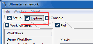
→ Activate the Explore perspective.

The Explore perspective appears. All algorithm evaluation is carried out in this perspective.

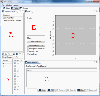
A The project list. Here, you select the project you want to evaluate.

B The currently selected filter. Remember that the parameter/value selections mentioned in the previous lesson. These selections can be used in this view as filters: only those parameters and values you choose are used in the evaluation. This enables you to play with the parameter settings to find interesting parameterizations.

C This view displays the parameterization that is considered optimal with respect to the currently active filter. It is currently empty because we didn't tell the Ultimate Framework the k parameter (see below).

D The performance plot. This view displays the performance curves of your algorithm.

E The parameter list. Here, you choose the parameter which shall be visualized by the X-axis of the performance plot.

We want to visualize the parameter setting for x and y that maximizes the objective function of SimpleProgram, i.e., leads to an optimal evaluation.

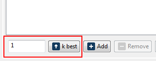
→ Enter the value 1 in the edit box at the bottom of C and click the k best button.

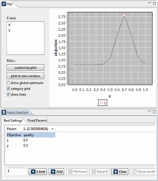Note the best setting for x (0.7) and y (0.3), displayed in the Best settings table (C). The performance plot now shows the complete performance curve for parameter x and emphasizes the optimal value, which is the peak at 0.7. The parameter list (E) enables us to choose between x and y.

→ Let us study the y parameter. In the parameter list (E), select y. Then, enter 4 in the edit box at the bottom of C and click the k best button.

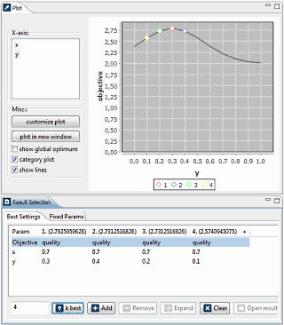From the best settings table, we now can tell that the best value for the x parameter is constantly 0.7 within the best 4 settings, but the values for y vary between 0.1 and 0.4, with 0.3 being the optimal setting. If you click on the column headers in the table, the performance plot will select the corresponding data point and highlight it.

If you try other settings for k and click the k best button, the data points are added to the table. They do not replace the existing data points. If you want to replace the exiting data points, you have to click the Clear button first.